Google Search Interest Time Series example
Introduction Link to heading
This report explores monthly search interest in the term “Vacation” within the United States, using data from Google Trends spanning from 2004 to early 2024. The search interest values are scaled from 0 to 100, where 100 represents peak popularity for the term during the time period. Given the nature of vacation planning, the data naturally display strong annual seasonality—with peaks typically occurring during summer months—as well as a long-term trend that suggests evolving interest over time.
The objective of this analysis is to model and forecast future search interest using time series techniques. Two complementary approaches are considered. First, we apply a decomposition method, explicitly modeling the trend and seasonal components using regression, with an AR(1) process capturing residual autocorrelation. Second, we implement a SARIMA model, which incorporates both seasonal and non-seasonal differencing to address non-stationarity in a more automated fashion.
By comparing the performance and forecasts of both models, we aim to evaluate their ability to capture the structure of the series and provide accurate predictions. This type of modeling has practical implications for businesses, travel agencies, or policymakers aiming to anticipate consumer interest in vacation planning.
https://trends.google.com/trends/explore?date=all&geo=US&q=vacation&hl=en
plot(vac.ts, ylab = "Interest/Searches", main = "Google searches for term 'Vacation'")
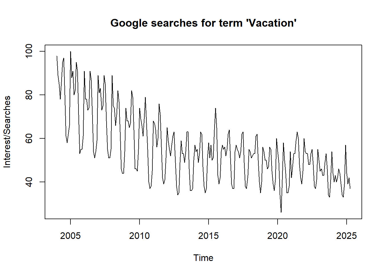 From the time series plot, we observe a long-term decreasing trend with regular seasonal fluctuations. Interest appears to fall steadily until around 2012, after which it levels off, suggesting a possible piecewise trend. Seasonal peaks and troughs indicate annual seasonality.
Trend and Seasonality Link to heading
We began by log-transforming the series to stabilize the variance. The log-transformed data showed both a nonlinear increasing trend and strong annual seasonality. A piecewise linear regression was used to model the trend, segmented at 2012, alongside a seasonal means model using monthly dummy variables.
To explicitly model the trend and seasonal components, we applied a piecewise linear regression model with monthly seasonal indicators to the log-transformed data. The trend was segmented around 2012, where a visible shift in growth occurred. The model used:
\(\log(y_t) = \beta_1 * T_1 + \beta_2 * T_2 + \gamma_{month(t)} + z_t\)
where \(z_t\) is the residual stationary component.
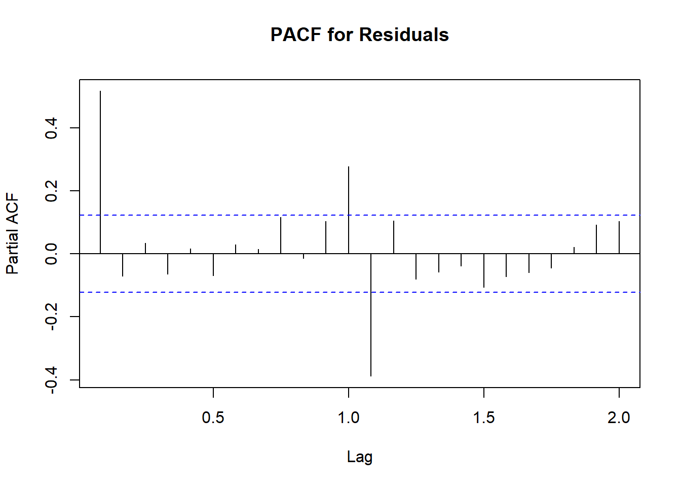
The residuals from this model exhibited autocorrelation consistent with an AR(1) structure. We therefore modeled the residual component as:
\(z_t = 0.542z_{t-1} +w_t\)
pacf(z1, main="PACF for Residuals")
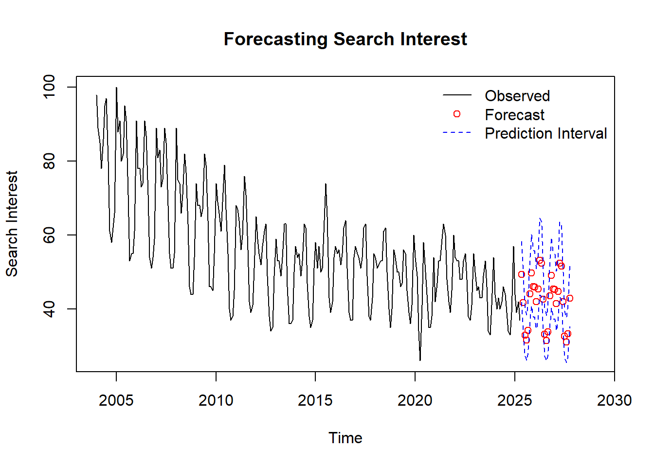
Combining the trend, seasonal effects, and AR(1) residual forecasts, we produced forecasts for the next 30 months. These were back-transformed to the original scale and included 95% prediction intervals. This approach offers a clear, interpretable decomposition of seasonal and long-term behavior.
plot(vac.ts, xlim=c(2004, 2029), main="Forecasting Search Interest", ylab = "Search Interest")
points(x1hat, col="red")
lines(pi.x.upper, lty=2, col="blue")
lines(pi.x.lower, lty=2, col="blue")
legend("topright",
       legend = c("Observed", "Forecast", "Prediction Interval"),
       col = c("black", "red", "blue"),
       lty = c(1, NA, 2),
       pch = c(NA, 1, NA),
       bty = "n")
SARIMA Modeling Link to heading
To provide a more compact, automated approach, we also modeled the log-transformed data using seasonal difference at lag 12 and regular differencing. The differenced series appeared stationary, and we compared three candidate models:
- SARIMA(1,1,0)(0,1,1)[12]
- SARIMA(0,1,1)(0,1,1)[12]
- SARIMA(1,1,1)(0,1,1)[12]
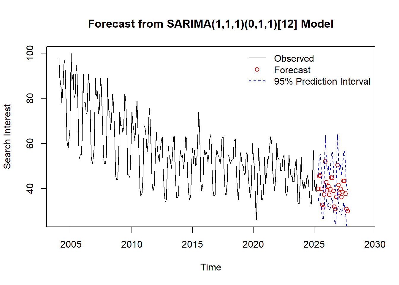
Based on AIC, the best model was:
\((1-0.648B)(1-B)(1-B^{12})x_t = (1-0.964B)(1-0.583B^{12})w_t\).
where \(w_t\) is white noise with \(\sigma^2 = 0.005\)
plot(vac.ts, xlim = c(2004, 2029), ylim = range(vac.ts, upper),
     main = "Forecast from SARIMA(1,1,1)(0,1,1)[12] Model", ylab = "Search Interest", xlab = "Time")

points(forecast_time, yhat, col = "red")

# prediction interval lines
lines(forecast_time, upper, col = "blue", lty = 2)
lines(forecast_time, lower, col = "blue", lty = 2)
legend("topright",
       legend = c("Observed", "Forecast", "95% Prediction Interval"),
       col = c("black", "red", "blue"),
       lty = c(1, NA, 2),
       pch = c(NA, 1, NA),
       bty = "n")
Model Comparision Link to heading
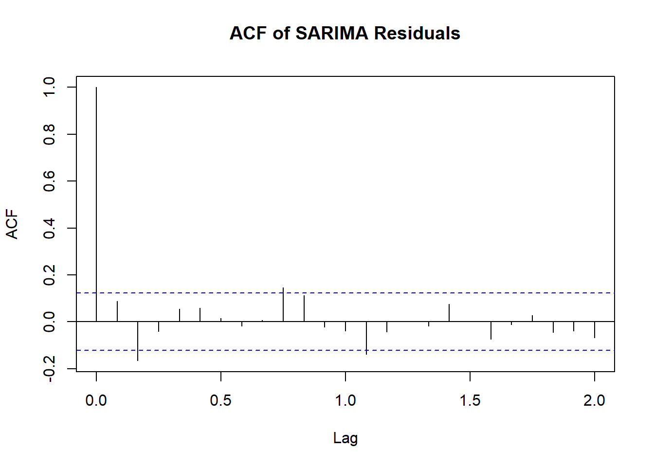
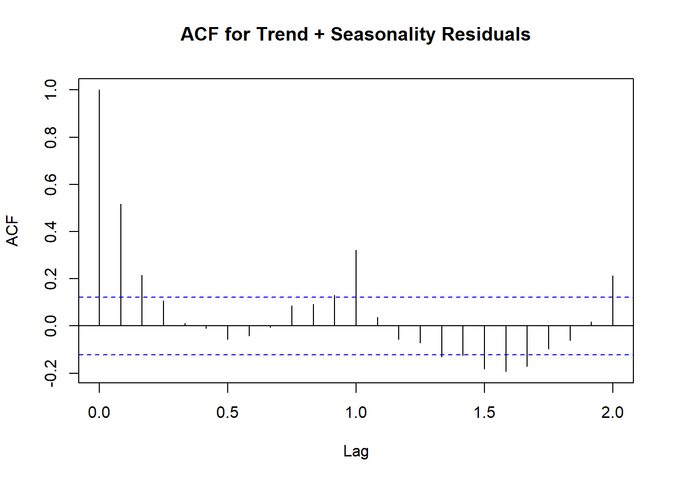
Both approaches adequately captured the trend and seasonality in the data. The regression + AR(1) model allows for clear interpretation of long-term behavior, while the SARIMA model fits slightly better and requires fewer parameters. Forecasts from both models were similar, but from the ACF plots of residuals confirm that the SARIMA model more effectively removed autocorrelations, indicating a better fit to the underlying process.
# ACF plot of residuals
acf(res_sarima, main = "ACF of SARIMA Residuals")
acf(z1, main = "ACF for Trend + Seasonality Residuals")
Conclusion Link to heading
This project analyzed Google search interest for the term “Vacation,” revealing strong yearly seasonality and a shifting long-term trend. We modeled the data using both a regression-based decomposition approach and a SARIMA model to capture and forecast this behavior.
While both methods produced similar forecasts, the SARIMA(1,1,1)(0,1,1)[12] model offered a better fit with fewer parameters. However, the regression approach provided clearer insight into structural components like trend changes and seasonal effects. Together, these models highlight how time series techniques can effectively describe and anticipate consumer interest patterns.