March-Madness-Analysis
Exploring the data Link to heading
Looking at historical champions Link to heading
Goal: Gain an understanding of what it takes for a team to win it all or even make it far in the tournament.
Exploring Seed and Net Rating as factors of team success leading into the tournament.
voilinPlot1
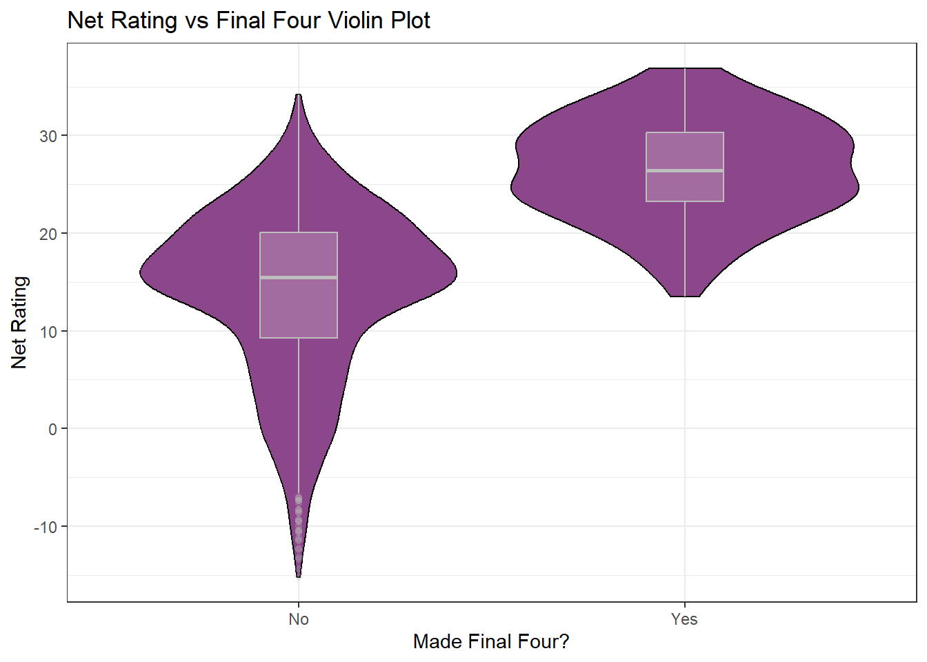 We can see teams that made the final four had on average a higher net rating than teams that did not.
p1 + p2 + plot_layout(axes = "collect")
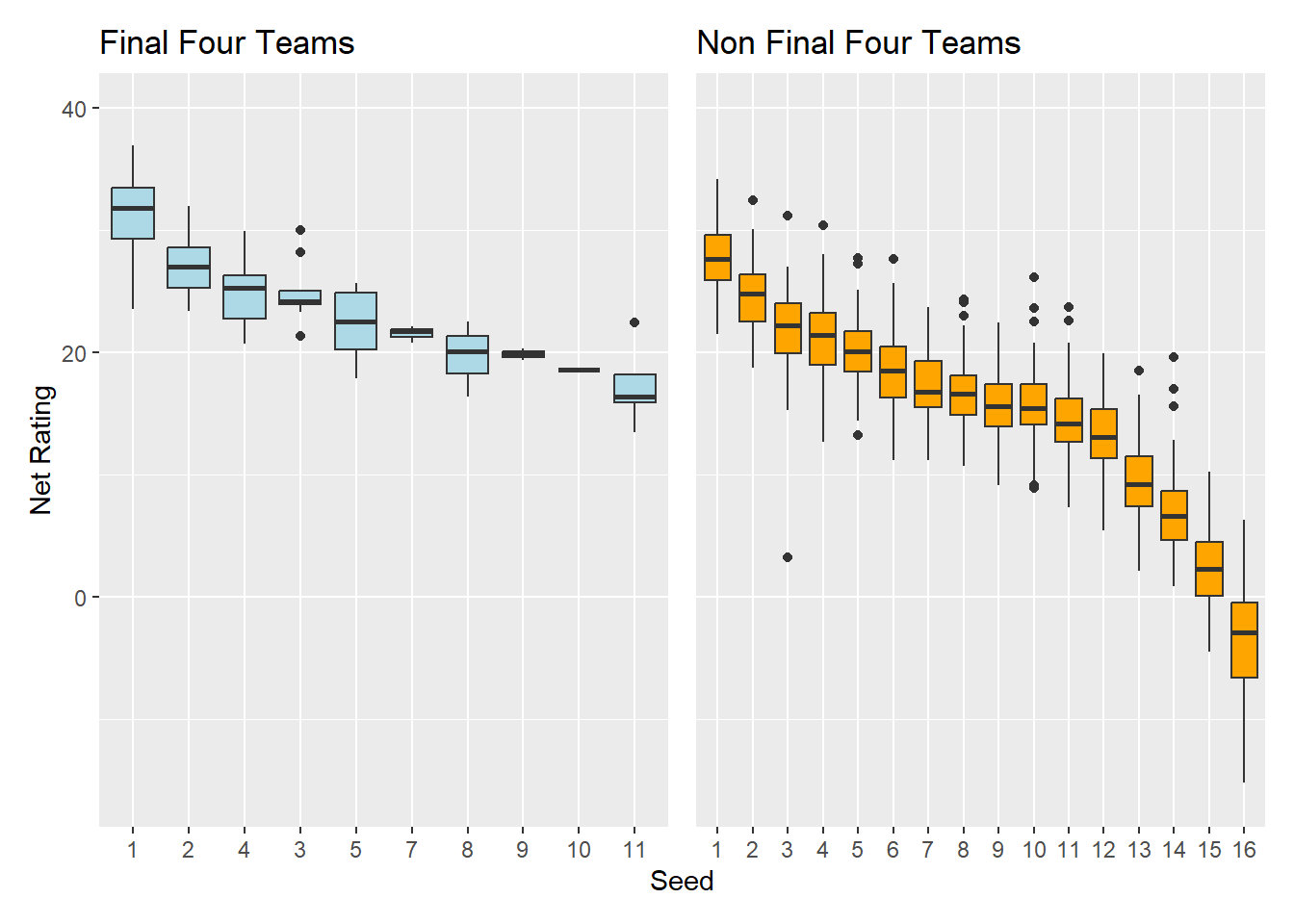
We can also see that in either case, teams with a higher seed (ie closer to 1) have on average a higher net rating than lower seeds, as well the lowest seed to make the final four (2002-2024) was an 11 seed, so we can assume it is not likely that an 12 or above seed will make the final four. Also notably a 6 seed has not made the final four since before 2002. Another thing of interest is 4 seed have a slightly higher median Net Rating than 3 seeds that made the final four.
In general Seed would be a good estimator of the which team is better as higher seeds tend to have higher net ratings.
f4.app.plot
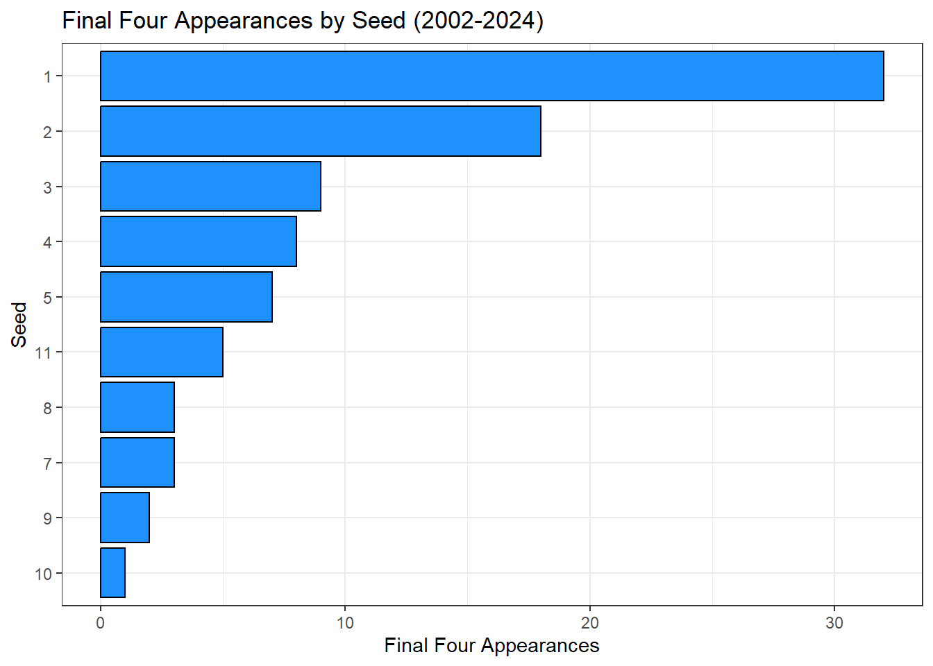
Interestingly the 11 seed has made the final four the 6th most out of any seed and no 6 seed has made it, since the 11 and 6 seed teams play first round this could be an indicator of common first round upsets.
p4
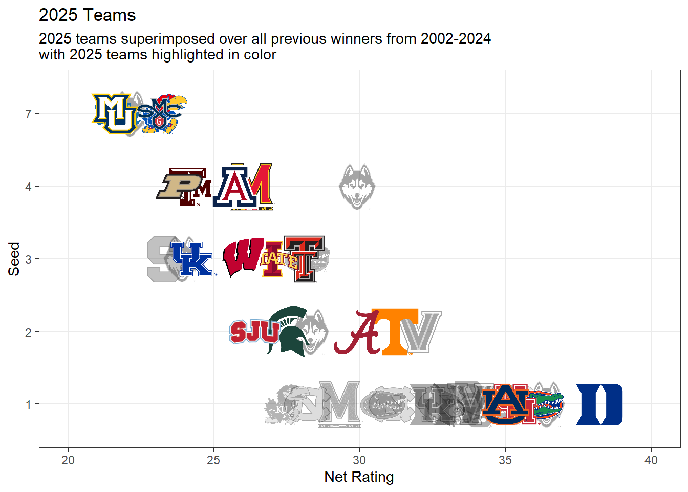 Here we can see that based off Net rating all 4 of the 1 seeds this year are above almost all previous winners, with notably Florida and Duke being the top 2 that are above all other teams.
We see that for the 2 seed Tennessee and Alabama compare well with other 2 seeds that have won before but are well below the avg for 1 seed and this years 1 seed.
All 3 seeds compare well with other 3 seeds that have won, with 2 previous team having a lower net rating than all 4 of this years teams.
There has been 1 7 seed champion and all 4 of the 7 seeds this year have similar if not higher net ratings than Uconn when they did it.
Here we can see that based off Net rating all 4 of the 1 seeds this year are above almost all previous winners, with notably Florida and Duke being the top 2 that are above all other teams.
We see that for the 2 seed Tennessee and Alabama compare well with other 2 seeds that have won before but are well below the avg for 1 seed and this years 1 seed.
All 3 seeds compare well with other 3 seeds that have won, with 2 previous team having a lower net rating than all 4 of this years teams.
There has been 1 7 seed champion and all 4 of the 7 seeds this year have similar if not higher net ratings than Uconn when they did it.
Needless to say 1 seeds seem far ahead of the board in chances to win, and this years 1 seeds are some of the strongest there has been.
Trapezoid of Success Link to heading
There is a new metric called the Trapezoid of success that guages team based off of pace and Net rating, the metric has successfully predicted the last 6 tournament winner.
trap.plot1
## Warning: Using the `size` aesthetic with geom_segment was deprecated in ggplot2 3.4.0.
## ℹ Please use the `linewidth` aesthetic instead.
## This warning is displayed once every 8 hours.
## Call `lifecycle::last_lifecycle_warnings()` to see where this warning was
## generated.
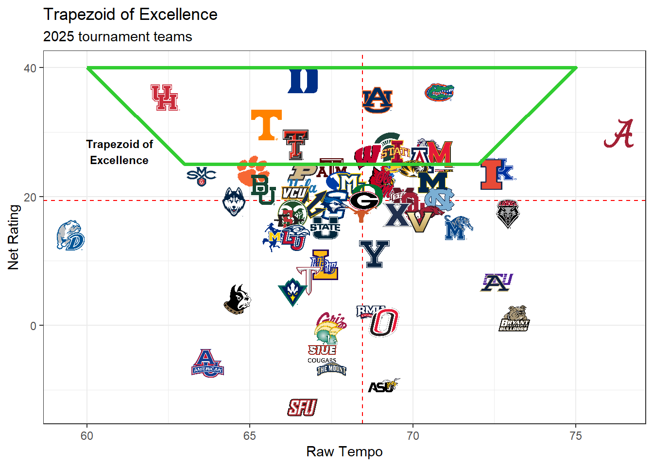
Credit to Ryan Hammer (@ryanhammer09 on twitter), the idea is that the ideal team in the tournament dont have to much of an extreme pace/tempo, but better teams are allowed more variation. According to Ryan teams within the trapezoid have historical success, and also high seeded teams that fall outside have a pattern of being eleminated early.
trap.plot2
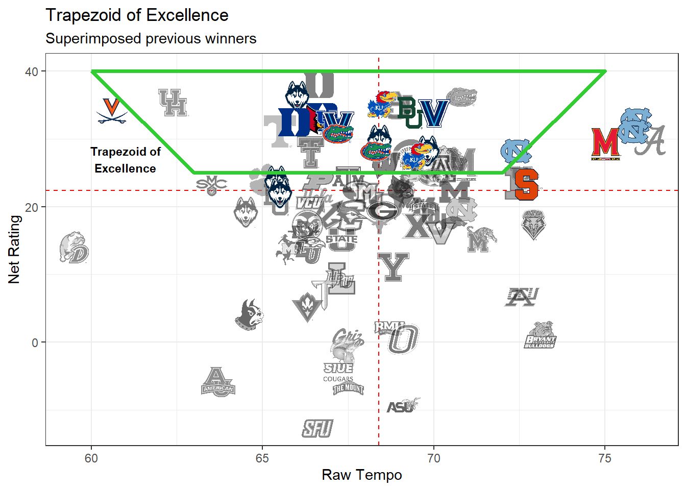
We can see the bulk of previous winners reside inside the trapezoid with some at the right Rating but higher tempo, and UVA at a lower tempo.
plot1 + plot2 + plot3 + plot4 +
  plot_layout(guides = "collect")
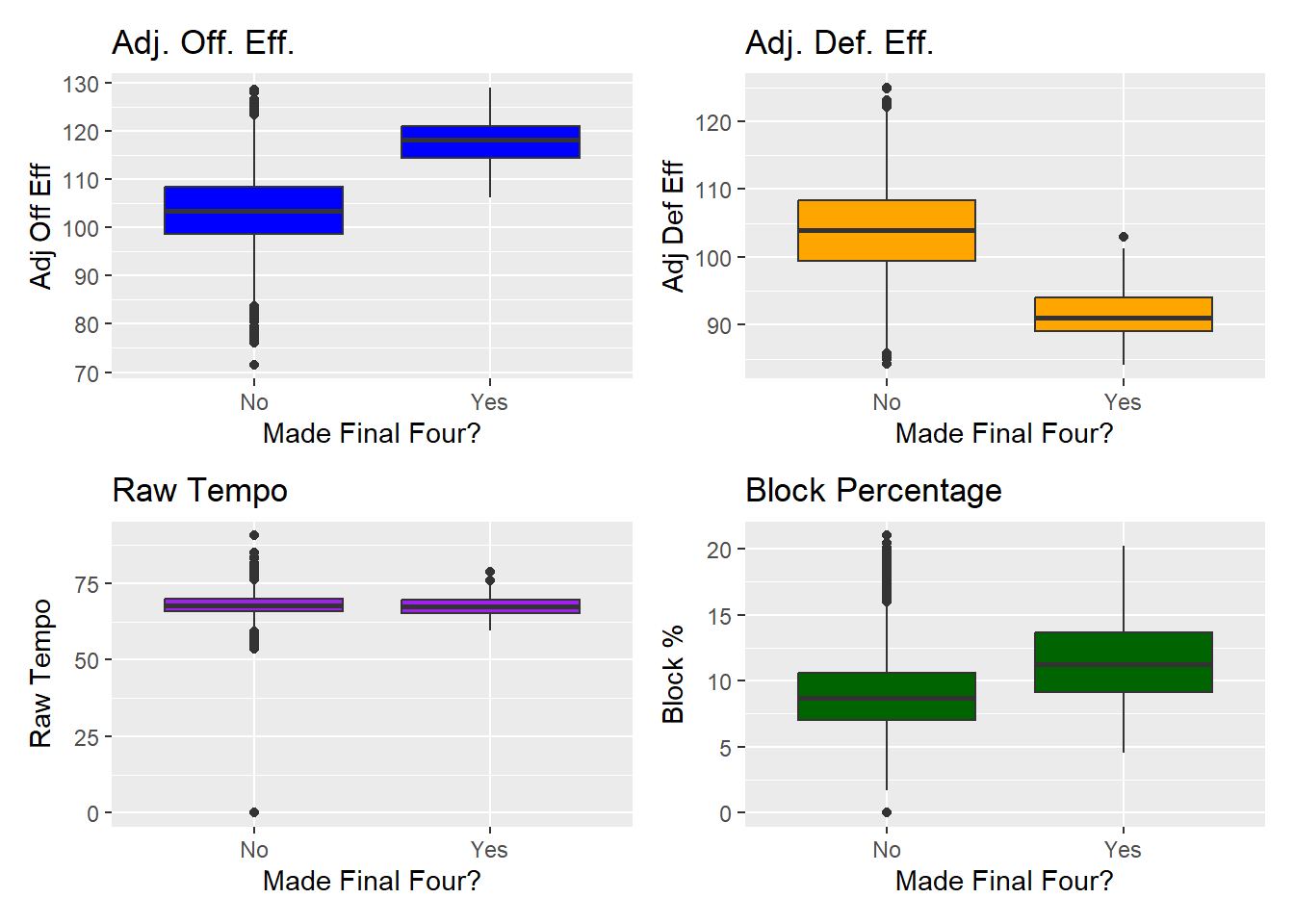
We can see from the plots above that there is a noticeable difference in Adjusted Offense and Defensive Eff. as well as Block percentage for teams that made it far in the tournament and teams that did not. Raw tempo did not have a difference but from the exploration plots of the trapezoid of excellence, it would be worthy to be used in the models.
(x3 | (x1/x2)) + plot_layout(guides = "collect")
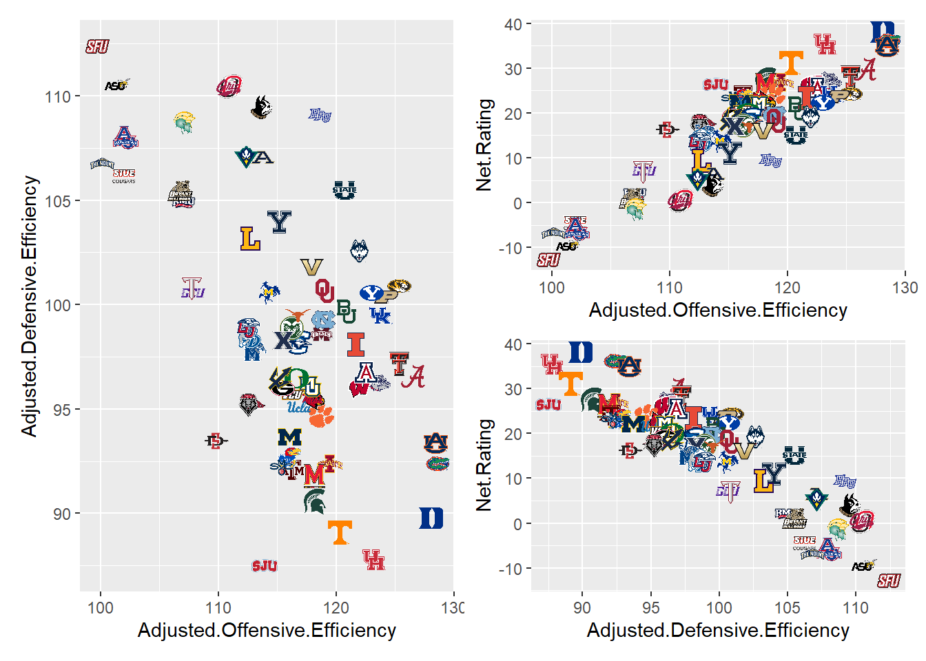
From these plots we can see that Net rating and adj off eff as well as adj def eff are highly correlated but the two eff stats are only less correlated with each other. So we will leave net rating out of the models and continue with using Adjusted.Offensive.Efficiency, Adjusted.Defensive.Efficiency, Raw.Tempo, and Block Percentage as covariates in further models.
Clustering Link to heading
With these clustering methods I aim to explore the patterns between previous tournament winner as well as the teams in this years tournament to see if there are any teams that stick out or are similar to previous winners.
d_eucli <- dist(subset, method = "euclidean") # using euclidean distance
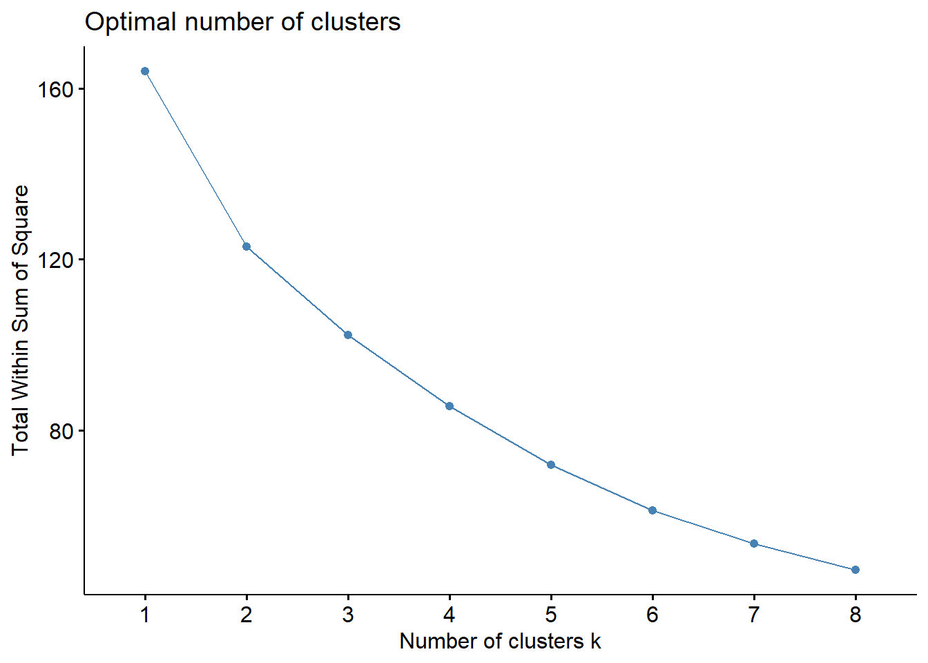
fviz_nbclust(scaled.subset, hcut, method = "wss", k.max = 8) # k could be 4-6
agnes.1 <- agnes(d_eucli, diss = T, metric = "euclidean")
pltree(agnes.1, main = "Agglomerative Euclidean Distance", hang = -1, xlab = "clustering by Raw.Tempo, Adj Off Eff, Adj Def Eff, Block %")
rect.hclust(agnes.1, k = 5, border = 2) # draw boxes around clusters
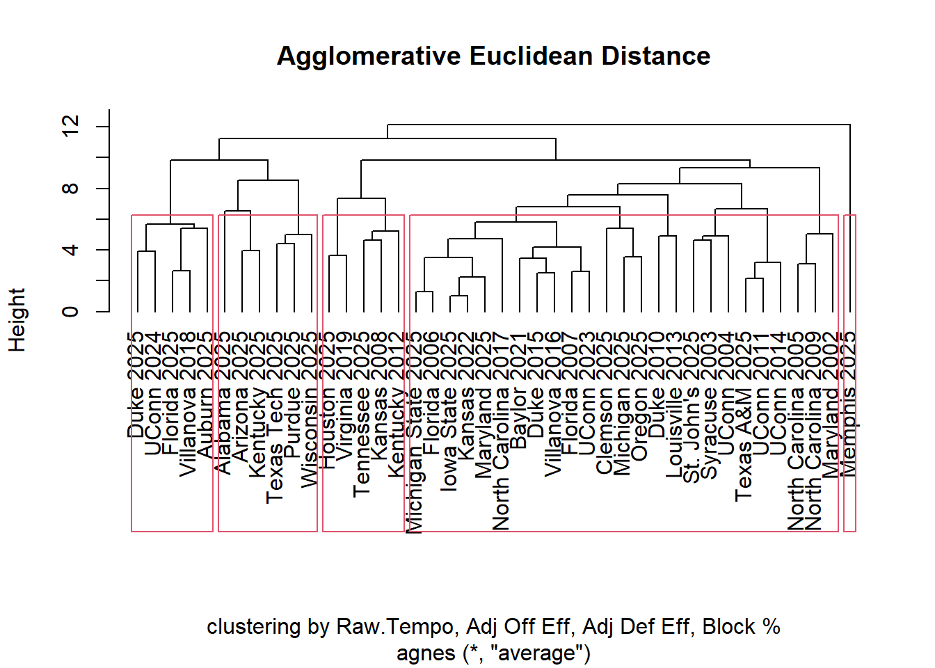
There isn’t a great “elbow” point here but 5 or 6 seems the most reasonably, I ended up choosing 5 clusters that can be seen in the dendrogram.
The dendrogram holds on previous winner as well as seeds 1-5 in this years tournament, we can see the left most cluster holds 3 of out 1 seeds this year and multiple other previous winners, the cluster to the right shows all teams from this years tournament implying there isn’t a strong connection to previous winners, the next cluster shows Houston and Tennessee with other winners, then we have a large collection of previous winners with this years teams, and finally a cluster of just Memphis.
We could possibly say Memphis, and the teams in cluster 2 might not have the best chances as they don’t compare with other teams that have won.
Kmeans clustering Link to heading
# How do lower seed cluster with past winners of higher seed
data252 <- filter(data25, Seed > 5)
dfinterest2 <- rbind(data252, success)
rownames(dfinterest2) <- paste(dfinterest2$Mapped.ESPN.Team.Name, dfinterest2$Season)
subset2 <- dfinterest2 %>%
  select(c("Raw.Tempo", "Adjusted.Offensive.Efficiency", "Adjusted.Defensive.Efficiency",
           "BlockPct"))

scaled.subset2 <- scale(subset2, center = T)
d_eucli <- dist(subset2, method = "euclidean")

fviz_nbclust(scaled.subset2, hcut, method = "wss", k.max = 8) # k = 5
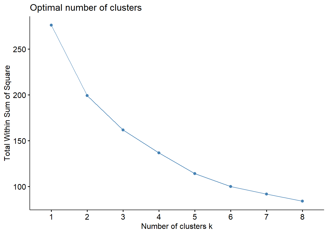
out.2 <- kmeans(scaled.subset2, centers = 6, nstart = 10)
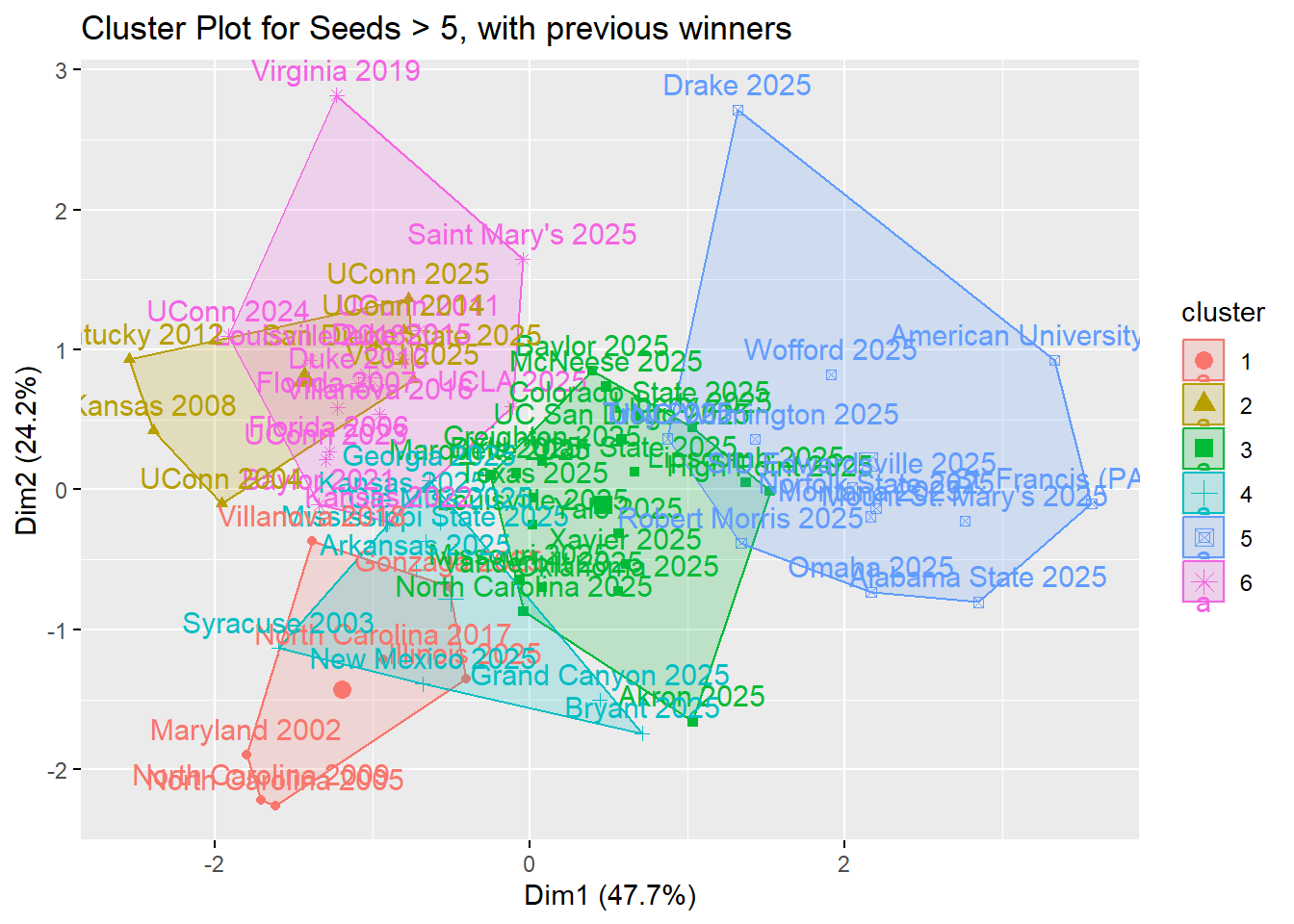
fviz_cluster(out.2, data = scaled.subset2) +
ggtitle("Cluster Plot for Seeds > 5, with previous winners")
out.3 <- kmeans(scaled.subset, centers = 5, nstart = 10)
fviz_cluster(out.3, data = scaled.subset) +
  ggtitle("Cluster Plot for Seeds <= 5, with previous winners")
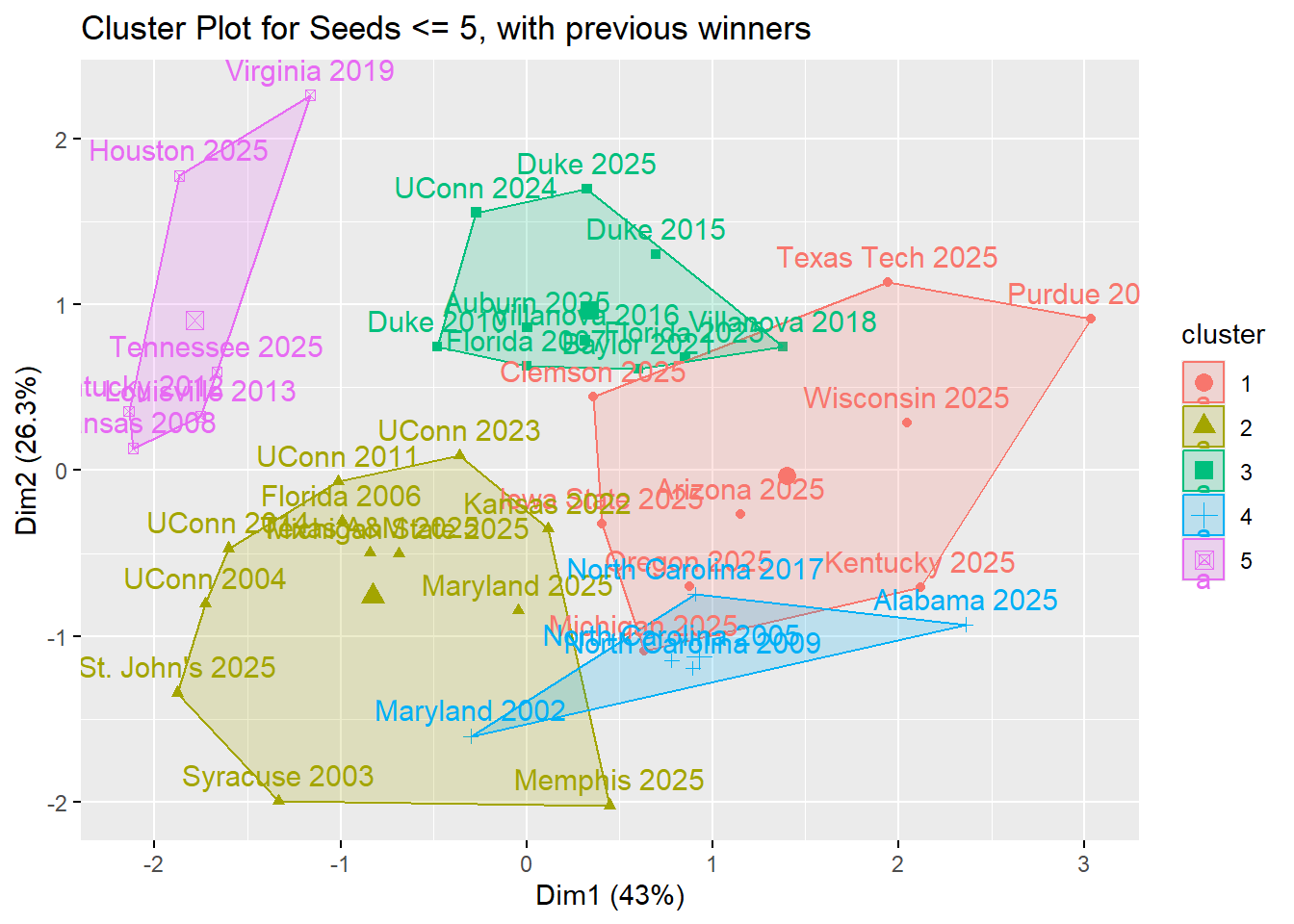
It appears all of the cluster 3 and 5 are teams that don’t compare well with previous champions, but the other clusters contain winners for the > 5 plot.
Notably in the <= 5 seed plot, Duke, Auburn and Florida are in their own cluster with previous winners, and we see im cluster 2 st johns and memphis are will winners as well.
set.seed(127)
scaled.subset3 <- scale(subset3 %>%
                          select(Raw.Tempo, Adjusted.Offensive.Efficiency,
                                 Adjusted.Defensive.Efficiency, BlockPct))
pca <- prcomp(scaled.subset3)

plot(pca$x[,1], pca$x[,2], xlab = "V1", ylab = "V2", pch = 16, col = "white",
     main = "PCA plot for 2025 teams and previous winners")

text(pca$x[,1], pca$x[,2], labels = rownames(scaled.subset3), cex = 0.66, col = labels)
legend("bottomleft",
       legend = c("Champions", "2025 & Seed < 5", "2025 & Seed >= 5"),
       col = c("lightseagreen", "black", "lightsalmon"),
       pch = 16)
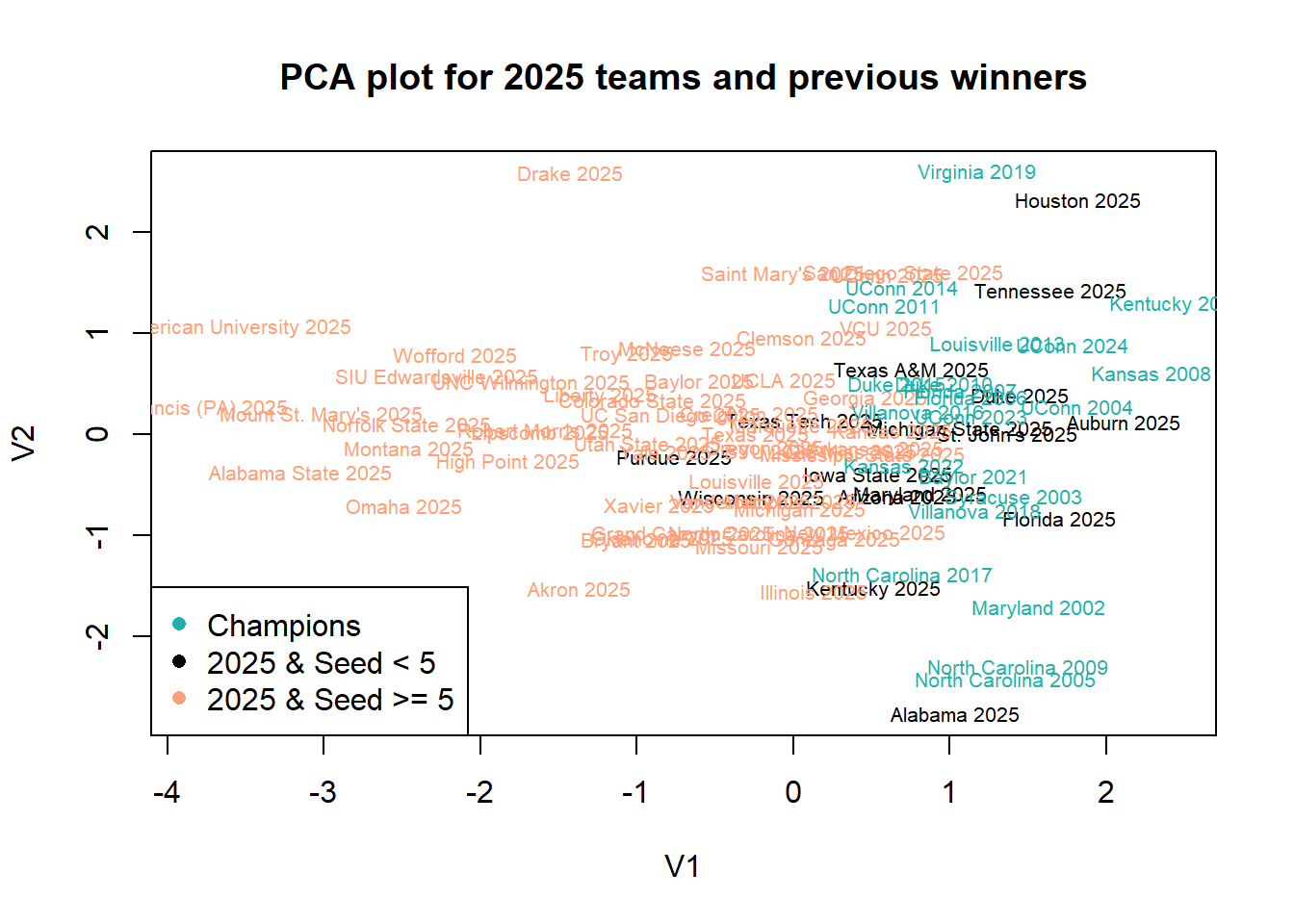 We can see that all previous champions fall somewhere between 0 and 2 on v1, we can see notable teams like Michigan St., Auburn, Texas A&M, Tennessee, Texas Tech, Kentucky, Maryland, Alabama and the 1 seed residing in there as well as a good amount of >= 5 seeded teams like Georgia, Illinois, VCU, and others.
Supervised Learning Link to heading
Moving on to some supervised learning techniques to help better examine every pick in this years bracket. To do this I’ll look into 2 different response variables that will be the indicator of success, firstly Seed and next if the team made the final four or not. I will use all of the march madness teams from 2002-2024 to train the models and then use those models to make predictions for the 2025 teams. The same variables of interest will be used as before.
The first model will be a Naive Bayes model, which essentially relies on using Bayes Theorem and assumes that all features of the model are independent of each other. So for this model is assumes tempo, offensive and defense efficiency, and block percentage or independent, and pick the seed/final four appearance with the highest probability given those stat lines.
# Naive Bayes
naiveSeed <- naiveBayes(as.factor(Seed) ~ Raw.Tempo + Adjusted.Offensive.Efficiency +
         Adjusted.Defensive.Efficiency + BlockPct, data = pastTeams)
naiveFF <- naiveBayes(as.factor(Final.Four.) ~ Raw.Tempo + Adjusted.Offensive.Efficiency +
         Adjusted.Defensive.Efficiency + BlockPct, data = pastTeams)
Next we will use a random forest model. Random forests models are made up of decision trees, each tree “learns” by splitting based on certain features (tempo,, block %, etc), and then picks the most common outcome based on those splits. The forest part comes into play since there are hundreds of the trees and all of them are averaged out to give us predictions.
# Random Forest
rfSeed <- randomForest(as.factor(Seed) ~ Raw.Tempo + Adjusted.Offensive.Efficiency +
         Adjusted.Defensive.Efficiency + BlockPct, data = pastTeams)
rfFF <- randomForest(as.factor(Final.Four.) ~ Raw.Tempo + Adjusted.Offensive.Efficiency +
         Adjusted.Defensive.Efficiency + BlockPct, data = pastTeams)
Next a Support Vector Machine (SVM), is a model which projects the data into a higher dimensional space and finds an optimal hyperplane to separate the data into different classes.
# SVM
svmSeed <- svm(Seed ~ Raw.Tempo + Adjusted.Offensive.Efficiency +
         Adjusted.Defensive.Efficiency + BlockPct,
         data = pastTeams,
         kernel = "radial")
svmFF <- svm(as.factor(Final.Four.) ~ Raw.Tempo + Adjusted.Offensive.Efficiency +
         Adjusted.Defensive.Efficiency + BlockPct,
         data = pastTeams,
         kernel = "radial")

predictors <- data25[, c("Raw.Tempo", "Adjusted.Offensive.Efficiency",
                         "Adjusted.Defensive.Efficiency", "BlockPct")]
preds <- predict(naiveSeed, data25)
preds <- factor(preds, levels = levels(data25$Seed))
confusionMatrix(preds, data25$Seed)
## Confusion Matrix and Statistics
##
##           Reference
## Prediction 1 2 3 4 5 6 7 8 9 10 11 12 13 14 15 16
##         1  4 4 0 0 0 0 0 0 0  0  0  0  0  0  0  0
##         2  0 0 1 3 1 1 1 1 0  0  0  0  0  0  0  0
##         3  0 0 3 1 0 3 0 3 2  2  1  0  1  0  0  0
##         4  0 0 0 0 0 0 0 0 0  0  0  0  0  0  0  0
##         5  0 0 0 0 0 0 0 0 1  1  2  0  0  0  0  0
##         6  0 0 0 0 2 0 3 0 0  0  0  0  0  0  0  0
##         7  0 0 0 0 0 0 0 0 1  0  1  2  0  0  0  0
##         8  0 0 0 0 1 0 0 0 0  1  1  0  0  0  0  0
##         9  0 0 0 0 0 0 0 0 0  0  0  0  0  0  0  0
##         10 0 0 0 0 0 0 0 0 0  0  0  0  0  0  0  0
##         11 0 0 0 0 0 0 0 0 0  0  0  2  0  0  0  0
##         12 0 0 0 0 0 0 0 0 0  0  1  0  1  1  0  0
##         13 0 0 0 0 0 0 0 0 0  0  0  0  1  1  0  0
##         14 0 0 0 0 0 0 0 0 0  0  0  0  1  1  1  0
##         15 0 0 0 0 0 0 0 0 0  0  0  0  0  0  1  0
##         16 0 0 0 0 0 0 0 0 0  0  0  0  0  1  2  6
##
## Overall Statistics
##
##                Accuracy : 0.2353
##                  95% CI : (0.1409, 0.3538)
##     No Information Rate : 0.0882
##     P-Value [Acc > NIR] : 0.0002284
##
##                   Kappa : 0.1834
##
##  Mcnemar's Test P-Value : NA
##
## Statistics by Class:
##
##                      Class: 1 Class: 2 Class: 3 Class: 4 Class: 5 Class: 6
## Sensitivity           1.00000  0.00000  0.75000  0.00000  0.00000  0.00000
## Specificity           0.93750  0.87500  0.79688  1.00000  0.93750  0.92188
## Pos Pred Value        0.50000  0.00000  0.18750      NaN  0.00000  0.00000
## Neg Pred Value        1.00000  0.93333  0.98077  0.94118  0.93750  0.93651
## Prevalence            0.05882  0.05882  0.05882  0.05882  0.05882  0.05882
## Detection Rate        0.05882  0.00000  0.04412  0.00000  0.00000  0.00000
## Detection Prevalence  0.11765  0.11765  0.23529  0.00000  0.05882  0.07353
## Balanced Accuracy     0.96875  0.43750  0.77344  0.50000  0.46875  0.46094
##                      Class: 7 Class: 8 Class: 9 Class: 10 Class: 11 Class: 12
## Sensitivity           0.00000  0.00000  0.00000   0.00000   0.00000   0.00000
## Specificity           0.93750  0.95312  1.00000   1.00000   0.96774   0.95312
## Pos Pred Value        0.00000  0.00000      NaN       NaN   0.00000   0.00000
## Neg Pred Value        0.93750  0.93846  0.94118   0.94118   0.90909   0.93846
## Prevalence            0.05882  0.05882  0.05882   0.05882   0.08824   0.05882
## Detection Rate        0.00000  0.00000  0.00000   0.00000   0.00000   0.00000
## Detection Prevalence  0.05882  0.04412  0.00000   0.00000   0.02941   0.04412
## Balanced Accuracy     0.46875  0.47656  0.50000   0.50000   0.48387   0.47656
##                      Class: 13 Class: 14 Class: 15 Class: 16
## Sensitivity            0.25000   0.25000   0.25000   1.00000
## Specificity            0.98438   0.96875   1.00000   0.95161
## Pos Pred Value         0.50000   0.33333   1.00000   0.66667
## Neg Pred Value         0.95455   0.95385   0.95522   1.00000
## Prevalence             0.05882   0.05882   0.05882   0.08824
## Detection Rate         0.01471   0.01471   0.01471   0.08824
## Detection Prevalence   0.02941   0.04412   0.01471   0.13235
## Balanced Accuracy      0.61719   0.60938   0.62500   0.97581
Looking at naive Bayes model, we can see the model’s accuracy is low, although higher than randomly guessing, but really struggles at predicting the middle seeded teams. To combat this I split the teams into three groups of high, medium and bottom seeded teams and will have the Bayes model and KNN model predicted these grouping, which will hopefully share some insight into what “bubble” teams are closer to higher ranking teams or bottom teams.
naiveSeed2 <- naiveBayes(as.factor(SeedGroup) ~ Raw.Tempo + Adjusted.Offensive.Efficiency +
         Adjusted.Defensive.Efficiency + BlockPct, data = pastTeams)
KNN or k’th nearest neighbor, is an algorithm which uses proximity to make classifications or predictions about the grouping of an individual points.
# KNN
train_X <- pastTeams[, c("Raw.Tempo", "Adjusted.Offensive.Efficiency",
                         "Adjusted.Defensive.Efficiency", "BlockPct")]
test_X <- data25[, c("Raw.Tempo", "Adjusted.Offensive.Efficiency",
                       "Adjusted.Defensive.Efficiency", "BlockPct")]

train_Y <- pastTeams$SeedGroup

knnSeed <- knn(train = train_X, test = test_X, cl = train_Y, k = 4)
Looking back at some of my picks the data did not support:
Lipscomb beating Iowa state, all models and clustering had Lipscomb as a bottom tier team and Iowa St. as a top team if not a 1 seed.
Uconn snuck into some of the models top tiers while Oklahoma appeared nothing but average, Uconn was the better team and I picked off who I didn’t want to win it all again, although the teams were probably pretty well matched.
Grand Canyon over Maryland, the models were accurate predicting grand canyon as a 13 seed and a bottom/middle team, while Maryland looked comparable to previous winners and was predicted high in seeding. This was nothing more of a recency bias pick and I didn’t believe in Maryland after watching them lose to that team up north in the B1G tournament.
2 of the models predicted Arkansas as a 5 seed, although a middle seeded team, but they over predicted Kansas as well.
picking McNeese and Troy to win was nothing more than expecting madness, those choices were not supported here.
As for the final four, i predicted Florida and duke, which which predicted to make it except SVM had Florida out of it, but everything here showed these 1 seeds were some of the best we’ve seen since 2002 so they should have made it, i still like my picks of Tennessee and Michigan State to make it and Tennessee was even predicted to reach final four in the Bayes model. As for the champion, it appears Duke was the best team ratings wise, but for some reason i liked Florida more and luckily i picked them.
These predictions can be seen in the table below.
table1
| Team | Actual Seed | Actual Final Four | Seed | Final Four | Group | Seed | Final Four | Seed | Final Four | Group |
|---|---|---|---|---|---|---|---|---|---|---|
| Duke | 1 | Yes | 1 | Yes | Top | 1 | Yes | 1 | Yes | Top |
| Florida | 1 | Yes | 1 | Yes | Top | 1 | Yes | 1 | No | Top |
| Houston | 1 | Yes | 1 | Yes | Top | 1 | Yes | 1 | Yes | Top |
| Auburn | 1 | Yes | 1 | Yes | Top | 1 | Yes | 1 | No | Top |
| Tennessee | 2 | No | 1 | Yes | Top | 1 | No | 1 | No | Top |
| Alabama | 2 | No | 1 | No | Top | 1 | Yes | 1 | No | Top |
| Michigan State | 2 | No | 1 | No | Top | 1 | No | 2 | No | Top |
| St. John's | 2 | No | 1 | No | Top | 2 | No | 1 | No | Top |
| Texas Tech | 3 | No | 3 | No | Top | 2 | No | 2 | No | Top |
| Iowa State | 3 | No | 2 | No | Top | 1 | No | 1 | No | Top |
| Wisconsin | 3 | No | 3 | No | Top | 2 | No | 3 | No | Top |
| Kentucky | 3 | No | 3 | No | Top | 2 | No | 3 | No | Top |
| Maryland | 4 | No | 2 | No | Top | 1 | No | 2 | No | Top |
| Arizona | 4 | No | 2 | No | Top | 2 | No | 2 | No | Top |
| Texas A&M | 4 | No | 2 | No | Top | 2 | No | 2 | No | Top |
| Purdue | 4 | No | 3 | No | Top | 3 | No | 3 | No | Top |
| Clemson | 5 | No | 2 | No | Middle | 4 | No | 2 | No | Top |
| Michigan | 5 | No | 6 | No | Middle | 3 | No | 3 | No | Middle |
| Oregon | 5 | No | 6 | No | Middle | 8 | No | 6 | No | Middle |
| Memphis | 5 | No | 8 | No | Middle | 11 | No | 11 | No | Middle |
| Missouri | 6 | No | 3 | No | Top | 3 | No | 3 | No | Top |
| Illinois | 6 | No | 3 | No | Top | 3 | No | 3 | No | Top |
| BYU | 6 | No | 3 | No | Top | 3 | No | 3 | No | Middle |
| Ole Miss | 6 | No | 2 | No | Middle | 4 | No | 4 | No | Middle |
| Kansas | 7 | No | 2 | No | Top | 4 | No | 4 | No | Top |
| Saint Mary's | 7 | No | 6 | No | Middle | 3 | No | 3 | No | Middle |
| UCLA | 7 | No | 6 | No | Middle | 3 | No | 5 | No | Middle |
| Marquette | 7 | No | 6 | No | Middle | 7 | No | 5 | No | Middle |
| Gonzaga | 8 | No | 3 | No | Top | 2 | No | 2 | No | Top |
| Louisville | 8 | No | 2 | No | Middle | 2 | No | 3 | No | Top |
| Mississippi State | 8 | No | 3 | No | Middle | 5 | No | 4 | No | Top |
| UConn | 8 | No | 3 | No | Top | 3 | No | 3 | No | Middle |
| Baylor | 9 | No | 3 | No | Middle | 3 | No | 3 | No | Top |
| Georgia | 9 | No | 5 | No | Middle | 5 | No | 5 | No | Middle |
| Creighton | 9 | No | 7 | No | Middle | 10 | No | 6 | No | Middle |
| Oklahoma | 9 | No | 3 | No | Middle | 3 | No | 8 | No | Middle |
| Arkansas | 10 | No | 5 | No | Middle | 7 | No | 5 | No | Middle |
| New Mexico | 10 | No | 8 | No | Middle | 12 | No | 4 | No | Middle |
| Vanderbilt | 10 | No | 3 | No | Middle | 7 | No | 11 | No | Middle |
| Utah State | 10 | No | 3 | No | Middle | 10 | No | 10 | No | Middle |
| VCU | 11 | No | 5 | No | Middle | 5 | No | 5 | No | Middle |
| North Carolina | 11 | No | 3 | No | Middle | 3 | No | 3 | No | Middle |
| Texas | 11 | No | 7 | No | Middle | 5 | No | 7 | No | Middle |
| Xavier | 11 | No | 8 | No | Middle | 8 | No | 8 | No | Middle |
| San Diego State | 11 | No | 5 | No | Middle | 9 | No | 9 | No | Middle |
| Drake | 11 | No | 12 | No | Middle | 11 | No | 12 | No | Middle |
| UC San Diego | 12 | No | 7 | No | Middle | 6 | No | 6 | No | Middle |
| Colorado State | 12 | No | 7 | No | Middle | 6 | No | 10 | No | Middle |
| McNeese | 12 | No | 11 | No | Middle | 11 | No | 11 | No | Middle |
| Liberty | 12 | No | 11 | No | Middle | 11 | No | 11 | No | Middle |
| Yale | 13 | No | 12 | No | Middle | 12 | No | 12 | No | Middle |
| High Point | 13 | No | 3 | No | Bottom | 15 | No | 15 | No | Middle |
| Grand Canyon | 13 | No | 13 | No | Middle | 14 | No | 13 | No | Bottom |
| Akron | 13 | No | 14 | No | Bottom | 13 | No | 13 | No | Bottom |
| Lipscomb | 14 | No | 12 | No | Bottom | 13 | No | 12 | No | Middle |
| Troy | 14 | No | 13 | No | Middle | 12 | No | 14 | No | Bottom |
| UNC Wilmington | 14 | No | 14 | No | Bottom | 15 | No | 15 | No | Bottom |
| Montana | 14 | No | 16 | No | Bottom | 16 | No | 16 | No | Bottom |
| Wofford | 15 | No | 16 | No | Bottom | 15 | No | 15 | No | Bottom |
| Robert Morris | 15 | No | 15 | No | Bottom | 15 | No | 15 | No | Bottom |
| Bryant | 15 | No | 14 | No | Bottom | 14 | No | 14 | No | Bottom |
| Omaha | 15 | No | 16 | No | Bottom | 16 | No | 16 | No | Bottom |
| Norfolk State | 16 | No | 16 | No | Bottom | 16 | No | 16 | No | Bottom |
| SIU Edwardsville | 16 | No | 16 | No | Bottom | 16 | No | 16 | No | Bottom |
| American University | 16 | No | 16 | No | Bottom | 16 | No | 16 | No | Bottom |
| Mount St. Mary's | 16 | No | 16 | No | Bottom | 16 | No | 16 | No | Bottom |
| Alabama State | 16 | No | 16 | No | Bottom | 16 | No | 16 | No | Bottom |
| St. Francis (PA) | 16 | No | 16 | No | Bottom | 16 | No | 16 | No | Bottom |